台灣地理資訊

---

目錄

1. 總覽
2. GMT介紹及安裝
3. 網路資源及配套軟體
4. 第零章: 基本概念及默認值
5. 第一章: 製作地圖(地理投影法)
6. 第二章: XY散佈圖(其他投影法)
7. 第三章: 等高線圖及剖面
8. 第四章: 地形圖與色階
9. 第五章: 地震活動性與機制解
10. 第六章: 向量與速度場
11. 第七章: 台灣地理資訊
12. 第八章: 直方、圓餅、三元圖
13. 第九章: 三維空間視圖
14. 第十章: 地質圖

---

11. 台灣地理資訊

本章的目的較為特殊，其目的是提供讀者繪製台灣地區常用的地理資訊， 並不針對特定模組做詳細的闡述，只針對處理這些資料會用到的指令做必要的說明，所使用的資料可以從 交通網路資訊倉儲系統及 政府資料開放平台找到，下載後的檔案處理流程，包含轉換座標系統及 排版將不墜述，如想了解，歡迎聯繫我。

11.1 目的

本章將學習如何繪製

1. 交通系統(Traffic Network)
2. 行政邊界(Region Border)
3. 河川流域(Drainage Area)
4. 斷層分佈及型態(Fault System)
5. 人口密度(Population Density)

11.2 學習的指令與概念

• gmtconvert: 處理多區塊式文件
• gmtspatial: 地理空間中線和多邊形的操作
• makecpt: 製作色階檔
• psscale: 繪製色彩條
• pstext: 在圖上進行排版文字
• psxy: 繪製線、多邊形、符號
• awk及sed語法的示範

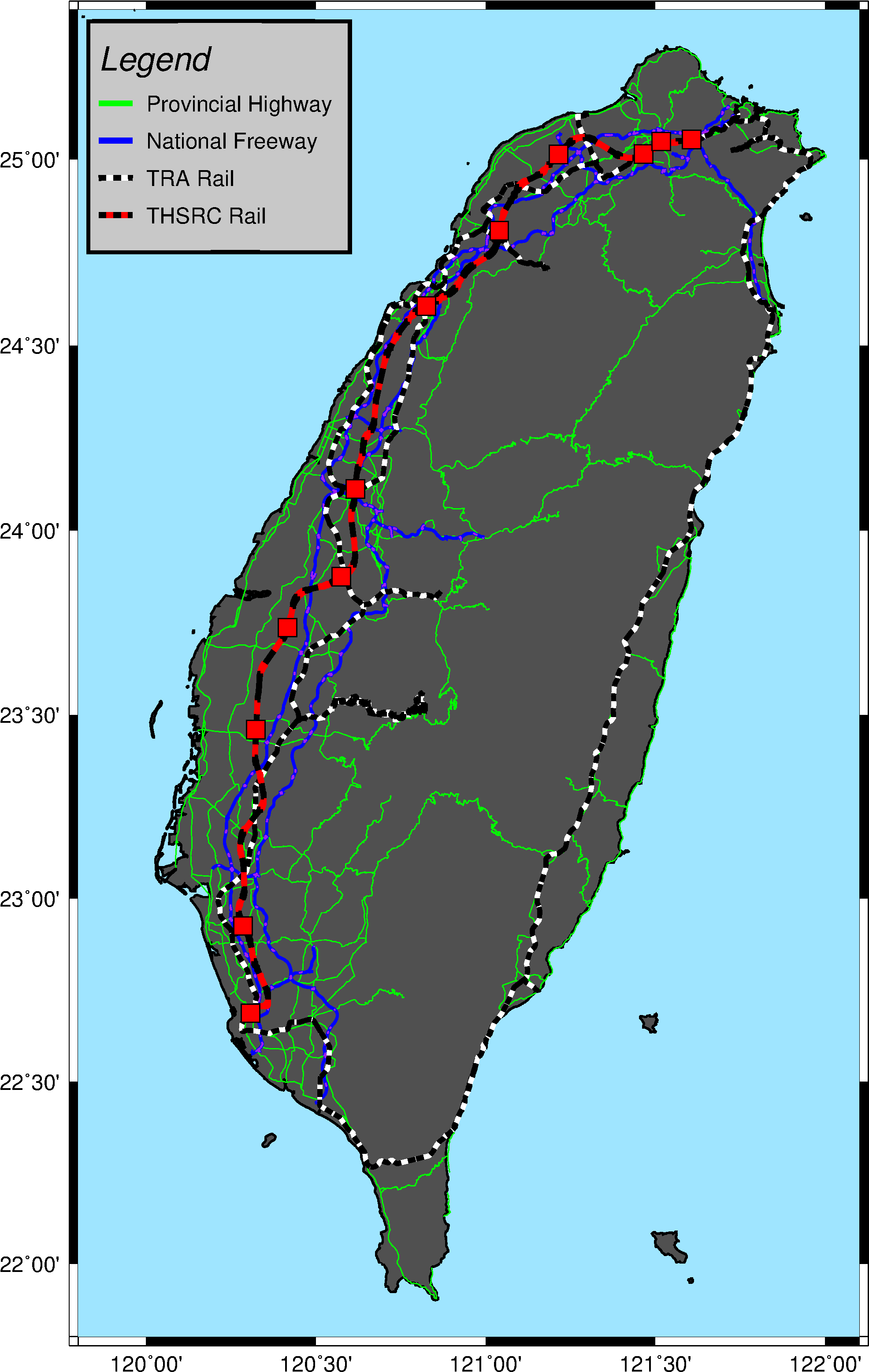
11.3 交通系統

首先示範台灣地區重要的交通道路系統，分別是省道(綠色)、國道(藍色)、台鐵(黑白相間)及高鐵(黑紅相間)。

使用的資料檔:

• 省道路線
• 國道路線
• 台鐵路縣
• 高鐵路縣

成果圖

批次檔

set ps=11_3_taiwan_road.ps
set data=D:\GMT_data\road\

# 1. road map
gmt psbasemap -R119.8/122.1/21.8/25.4 -JM15 -BWeSn -Ba -P -K > %ps%
gmt pscoast -R -JM -Df -W1 -G80 -S159/229/255 -K -O >> %ps%
gmt psxy %data%provincial_highway.gmt -R -JM -W.4,green -K -O >> %ps%
gmt psxy %data%national_freeway.gmt -R -JM -W1.5,blue -K -O >> %ps%
gmt psxy %data%national_freeway_attach.gmt -R -JM -W.7,purple -K -O >> %ps%
gmt psxy %data%TRA_rail.gmt -R -JM -W2.5,white -K -O >> %ps%
gmt psxy %data%TRA_rail.gmt -R -JM -W2.5,black,4_4:0p -K -O >> %ps%
gmt psxy %data%THSRC_rail.gmt -R -JM -W3,red -K -O >> %ps%
gmt psxy %data%THSRC_rail.gmt -R -JM -W3,black,8_8:0p -K -O >> %ps%
gmt psxy %data%THSRC_station.gmt -R -JM -Ss.5 -W.5 -Gred -K -O >> %ps%

# 2. legend set
echo 119.83 25.37 > tmp
echo 119.83 24.75 >> tmp
echo 120.60 24.75 >> tmp
echo 120.60 25.37 >> tmp
gmt psxy tmp -R -JM -W2 -L -G200 -K -O >> %ps%
echo 119.86 25.27 Legend | gmt pstext -R -JM -F+f18,2+jML -K -O >> %ps%
echo 119.86 25.15 > tmp
echo 119.96 25.15 >> tmp
gmt psxy tmp -R -JM -W3,green -K -O >> %ps%
echo 120.00 25.15 Provincial Highway | gmt pstext -R -JM -F+f12+jML -K -O >> %ps%
echo 119.86 25.05 > tmp
echo 119.96 25.05 >> tmp
gmt psxy tmp -R -JM -W3,blue -K -O >> %ps%
echo 120.00 25.05 National Freeway | gmt pstext -R -JM -F+f12+jML -K -O >> %ps%
echo 119.86 24.95 > tmp
echo 119.96 24.95 >> tmp
gmt psxy tmp -R -JM -W3,white -K -O >> %ps%
gmt psxy tmp -R -JM -W3,black,4_4:0p -K -O >> %ps%
echo 120.00 24.95 TRA Rail | gmt pstext -R -JM -F+f12+jML -K -O >> %ps%
echo 119.86 24.85 > tmp
echo 119.96 24.85 >> tmp
gmt psxy tmp -R -JM -W3,red -K -O >> %ps%
gmt psxy tmp -R -JM -W3,black,4_4:0p -K -O >> %ps%
echo 120.00 24.85 THSRC Rail | gmt pstext -R -JM -F+f12+jML -K -O >> %ps%

gmt psxy -R -J -T -O >> %ps%
gmt psconvert %ps% -Tg -A -P
del tmp*

學習到的指令:

• gmt psxy %data%TRA_rail.gmt -R -JM -W2.5,black,4_4:0p -K -O >> %ps%
  • 之前有提到-W寬度,顏色,樣式，其中樣式可以用-,.符號來繪製虛線， 這邊使用4_4:0p，數字分別對應虛線長度、虛線間隔長度、起始位置偏移， 來詳細控制虛線的屬性。

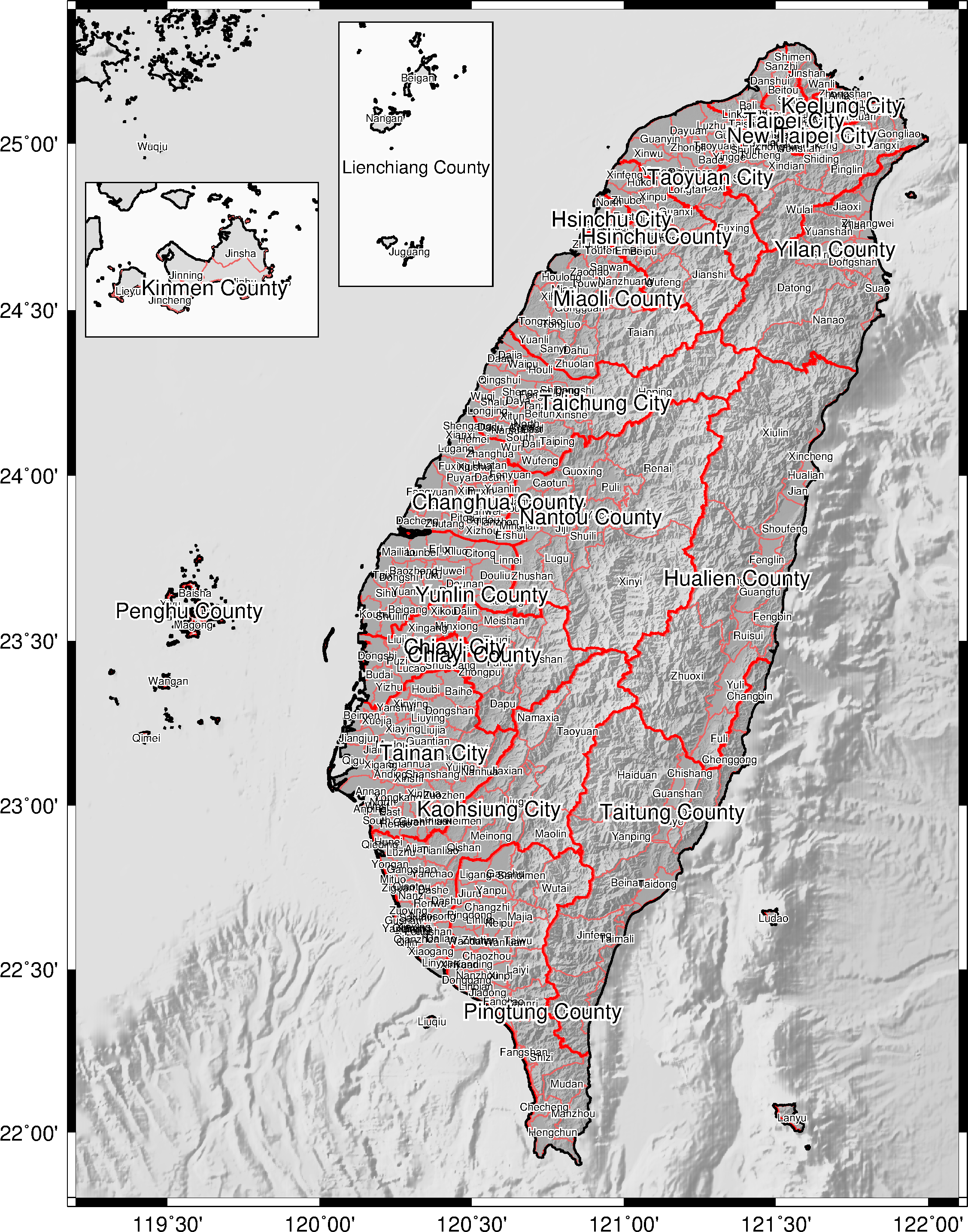
11.4 行政邊界

示範如何繪製鄉鎮市的行政邊界，並把各鄉鎮市的名字標記上去。

使用的資料檔:

• 都市邊界
• 鄉鎮邊界

成果圖

批次檔

set ps=11_4_region_border.ps
set data=D:\GMT_data\
set cpt=gebco.cpt

# Taiwan
gmt psbasemap -R119.2/122.1/21.8/25.4 -Jm6 -BWeSn -Ba -P -K > %ps%
gmt grdimage %data%tw_500_119.grd -R -Jm -C%cpt% -I%data%tw_500shad_119.grd -M -K -O >> %ps%
gmt pscoast -R -Jm -Df -Gc -K -O >> %ps%
gmt grdimage %data%tw_40.grd -R -Jm -C%cpt% -I%data%tw_40shad.grd -M -K -O >> %ps%
gmt psxy %data%country_2016.gmt -R -Jm -W.5,237/98/98 -K -O >> %ps%
gmt psxy %data%city_2016.gmt -R -Jm -W1,red -K -O >> %ps%
gmt pscoast -R -Jm -Df -Q -K -O >> %ps%
gmt pscoast -R -Jm -Df -W1 -K -O >> %ps%

gmt gmtspatial %data%country_2016.gmt -Q+p -o0,1 > tmp1
gmt gmtconvert %data%country_2016.gmt -L > tmp2
awk "NR==FNR{tmp1[NR]=$0; next} {print tmp1[FNR], $2,$3,$4}" tmp1 tmp2 > tmp
awk "{print $1,$2,$3}" tmp | gmt pstext -R -Jm -F+f6p=1p,white -K -O >> %ps%
awk "{print $1,$2,$3}" tmp | gmt pstext -R -Jm -F+f6p -K -O >> %ps%
gmt gmtspatial %data%city_2016.gmt -Q+p -o0,1 > tmp1
gmt gmtconvert %data%city_2016.gmt -L > tmp2
awk "NR==FNR{tmp1[NR]=$0; next} {print tmp1[FNR], $2,$3,$4}" tmp1 tmp2 > tmp
gmt pstext tmp -R -Jm -F+f12p=2p,white -K -O >> %ps%
gmt pstext tmp -R -Jm -F+f12p -K -O >> %ps%

# Kinmen
gmt psbasemap -R118.17/118.55/24.35/24.58 -Jm12 -Bwesn -B0 ^
-X.2 -Y17 -K -O --MAP_FRAME_TYPE=plain >> %ps%
gmt pscoast -R -Jm -Df -W1 -G220 -S250 -K -O >> %ps%
gmt pscoast -R -Jm -Df -Gc -K -O >> %ps%
gmt psxy %data%country_2016.gmt -R -Jm -W.5,237/98/98 -K -O >> %ps%
gmt pscoast -R -Jm -Df -Q -K -O >> %ps%

gmt gmtspatial %data%country_2016.gmt -Q+p -o0,1 > tmp1
gmt gmtconvert %data%country_2016.gmt -L > tmp2
awk "NR==FNR{tmp1[NR]=$0; next} {print tmp1[FNR], $2,$3,$4}" tmp1 tmp2 > tmp
awk "{print $1,$2,$3}" tmp | gmt pstext -R -Jm -F+f6p=1p,white -K -O >> %ps%
awk "{print $1,$2,$3}" tmp | gmt pstext -R -Jm -F+f6p -K -O >> %ps%
gmt gmtspatial %data%city_2016.gmt -Q+p -o0,1 > tmp1
gmt gmtconvert %data%city_2016.gmt -L > tmp2
awk "NR==FNR{tmp1[NR]=$0; next} {print tmp1[FNR], $2,$3,$4}" tmp1 tmp2 > tmp
gmt pstext tmp -R -Jm -F+f12p=2p,white -K -O >> %ps%
gmt pstext tmp -R -Jm -F+f12p -K -O >> %ps%

# Lienchiang
gmt psbasemap -R119.86/120.11/25.91/26.30 -Jm -Bwesn -B0 ^
-X5 -Y1 -K -O --MAP_FRAME_TYPE=plain >> %ps%
gmt pscoast -R -Jm -Df -W1 -G220 -S250 -K -O >> %ps%

gmt gmtspatial %data%country_2016.gmt -Q+p -o0,1 > tmp1
gmt gmtconvert %data%country_2016.gmt -L > tmp2
awk "NR==FNR{tmp1[NR]=$0; next} {print tmp1[FNR], $2,$3,$4}" tmp1 tmp2 > tmp
awk "{print $1,$2,$3}" tmp | gmt pstext -R -Jm -F+f6p=1p,white -K -O >> %ps%
awk "{print $1,$2,$3}" tmp | gmt pstext -R -Jm -F+f6p -K -O >> %ps%
gmt gmtspatial %data%city_2016.gmt -Q+p -o0,1 > tmp1
gmt gmtconvert %data%city_2016.gmt -L > tmp2
awk "NR==FNR{tmp1[NR]=$0; next} {print tmp1[FNR], $2,$3,$4}" tmp1 tmp2 > tmp
gmt pstext tmp -R -Jm -F+f10p=2p,white -D.7/-1 -K -O >> %ps%
gmt pstext tmp -R -Jm -F+f10p -D.7/-1 -K -O >> %ps%

gmt psxy -R -J -T -O >> %ps%
gmt psconvert %ps% -Tg -A -P
del tmp*

學習到的指令:

• gmtspatial -Q+p -o0,1從多區塊文件中算出質心位置。
  • -Q+p假設每個區塊文件中的資料都是封閉多邊形，並計算出質心位置。
  • -o0,1指定輸出第一欄(經度)和第二欄(緯度)。
• gmt gmtconvert -L從多區塊文件中提取檔頭資訊。
  • -L只輸出檔頭資訊。
• awk "NR==FNR{tmp1[NR]=$0; next} {print tmp1[FNR], $2,$3,$4}" 將經緯度及檔頭資訊中的縣市名稱合併成暫存檔，方便繪製。
• pstext -F+f6p=1p,white繪製文字邊框。
  • -F+f6p=1p,white中=號後面是相對文字大小的邊框寬度及顏色。

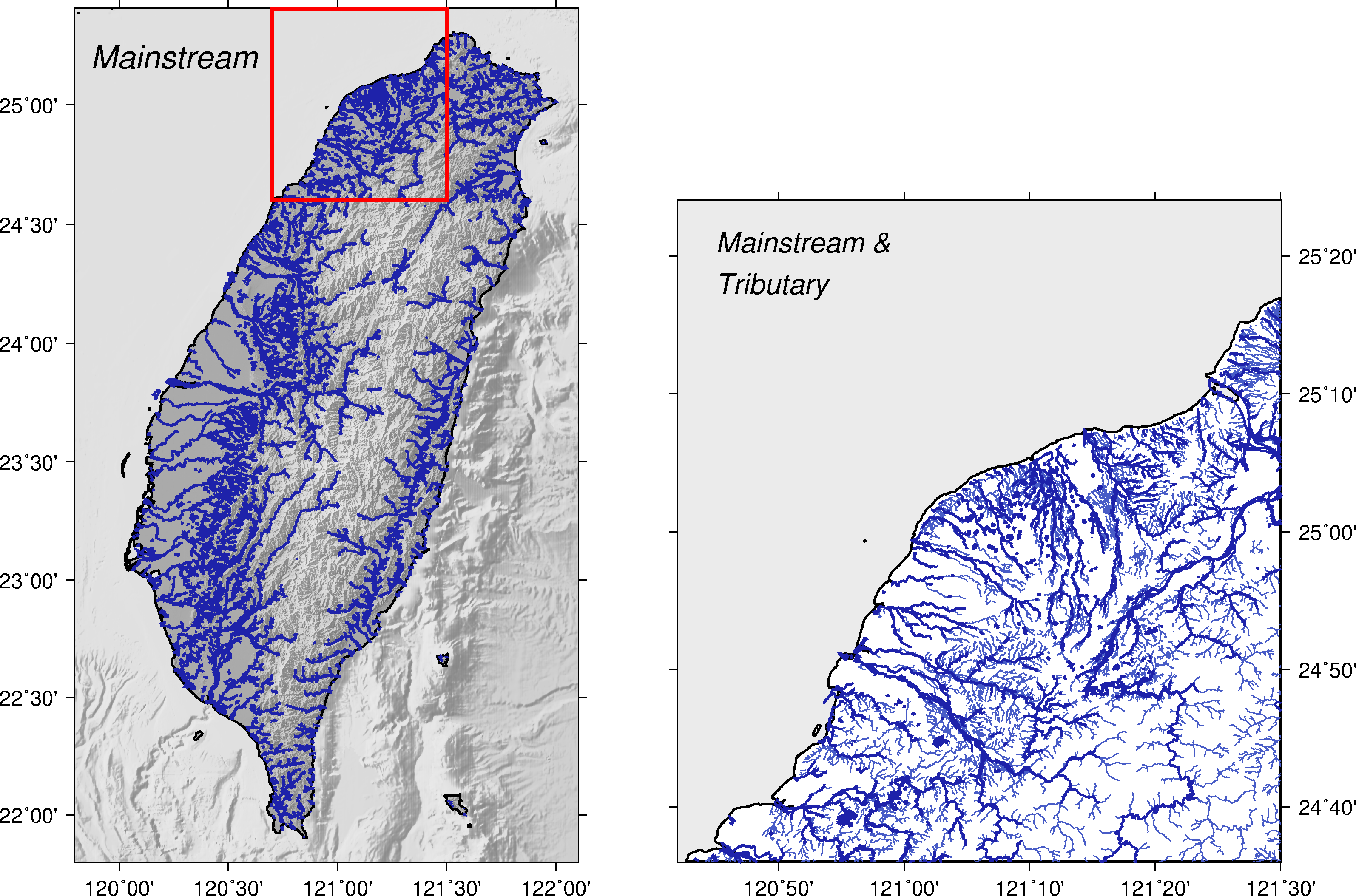
11.5 河川流域

由於pscoast的河川資料庫中並無包含台灣河川的資料，所以需要另外下載製作， 本節將分別繪製河川主流(Mainstream)流域圖及支流(Tributary)流域圖。

使用的資料檔:

• 河川主流資料
• 河川支流資料

成果圖

批次檔

set ps=11_5_drainage_area.ps
set data=D:\GMT_data\
set cpt=gebco.cpt

# mainstream
gmt gmtset MAP_FRAME_TYPE=plain
gmt psbasemap -R119.8/122.1/21.8/25.4 -JM10 -BWeSn -Ba -K > %ps%
gmt grdimage %data%tw_500_119.grd -R -JM -C%cpt% -I%data%tw_500shad_119.grd -M -K -O >> %ps%
gmt pscoast -R -JM -Df -Gc -K -O >> %ps%
gmt grdimage %data%tw_40.grd -R -JM -C%cpt% -I%data%tw_40shad.grd -M -K -O >> %ps%
gmt pscoast -R -JM -Df -Q -K -O >> %ps%
gmt pscoast -R -JM -Df -W1 -K -O >> %ps%
gmt psxy %data%taiwan_river_mainstream.gmt -R -JM -W1,30/34/170 -K -O >> %ps%
echo 119.87 25.2 Mainstream | gmt pstext -R -JM -F+f18p,2+jML -K -O >> %ps%
gmt psbasemap -R -JM -D120.7/121.5/24.6/25.4 -F+p2,red -K -O >> %ps%

# mainstream & tributary
gmt psbasemap -R120.7/121.5/24.6/25.4 -JM12 -BwESn -Ba -X12 -K -O >> %ps%
gmt pscoast -R -JM -Df -W1 -S235 -K -O >> %ps%
gmt psxy %data%taiwan_river_tributary.gmt -R -JM -W.5,72/92/199 -K -O >> %ps%
gmt psxy %data%taiwan_river_mainstream.gmt -R -JM -W1,30/34/170 -K -O >> %ps%
echo 120.75 25.35 Mainstream \046 | gmt pstext -R -JM -F+f16p,2+jML -K -O >> %ps%
echo 120.75 25.30 Tributary | gmt pstext -R -JM -F+f16p,2+jML -K -O >> %ps%

gmt psxy -R -J -T -O >> %ps%
gmt psconvert %ps% -Tg -A -P
del tmp* gmt.conf

學習到的指令:

• echo 120.75 25.35 Mainstream \046 | gmt pstext寫出特殊字元(&)。
  • \046可對應到&符號， 詳細內容請參考4-4特殊字元或符號。

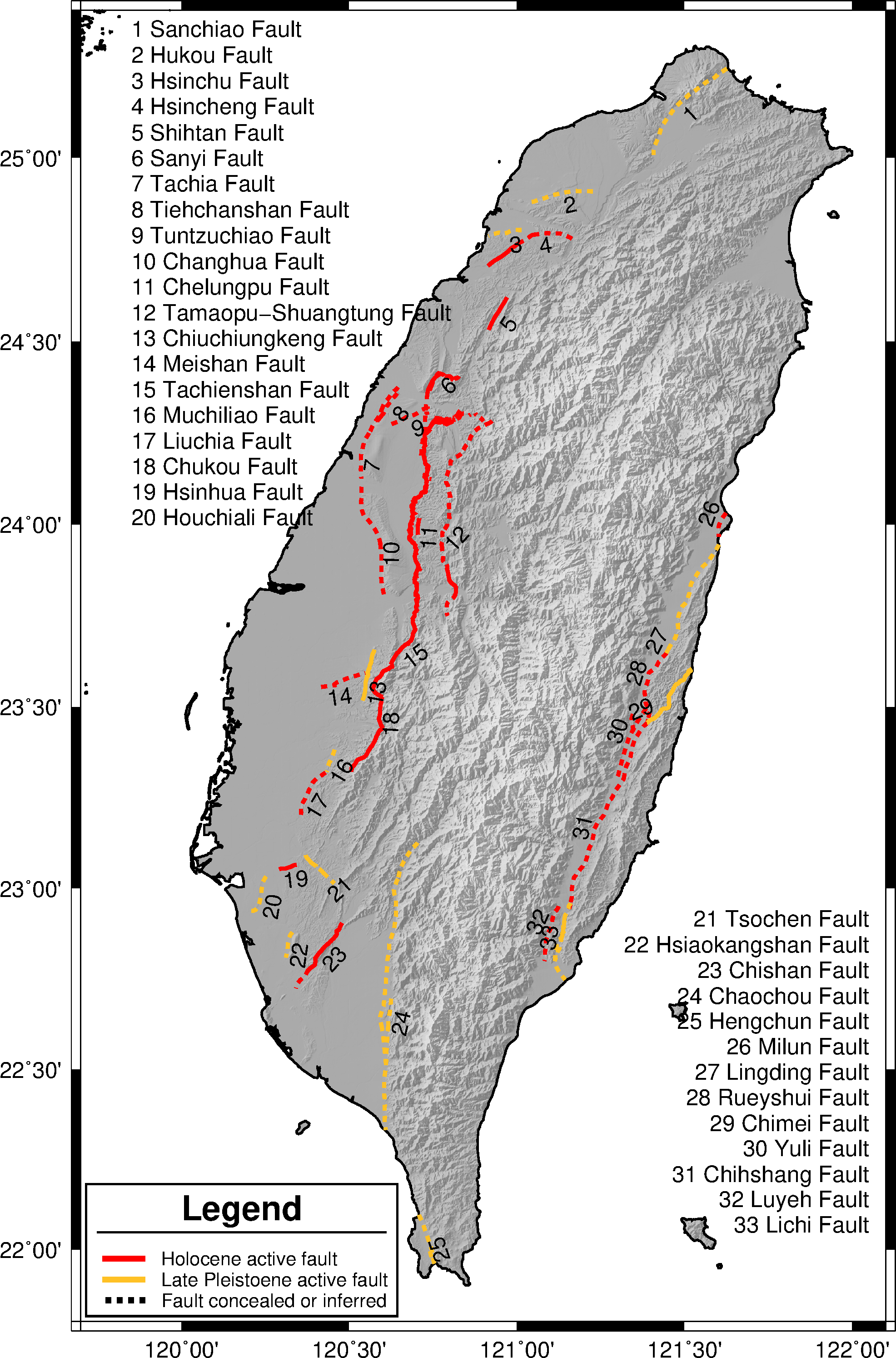
11.6 斷層分佈及型態

繪製由中央地質調查所提供的33條斷層分佈，並分類成第一類活動斷層、 第二類活動斷層及存疑、掩埋與否。

使用的資料檔:

• 斷層分佈資料
• 斷層編號

完成圖如下:

批次檔

set ps=11_6_cgs_fault.ps
set data=D:\GMT_data\
set cpt=gebco.cpt

# 1. topographic map
gmt psbasemap -R119.7/122.1/21.8/25.4 -JM15 -BWeSn -Ba -P -K > %ps%
gmt pscoast -R -JM -Df -Gc -K -O >> %ps%
gmt grdimage %data%tw_40.grd -R -JM -C%cpt% -I%data%tw_40shad.grd -M -K -O >> %ps%
gmt pscoast -R -JM -Df -Q -K -O >> %ps%
gmt pscoast -R -JM -Df -W1 -K -O >> %ps%

# 2. fault type
gmt psxy %data%CGS_fault.gmt -R -JM -Sqn1:+Lh+T"fault_label.dat" > tmp
gmt gmtconvert %data%CGS_fault.gmt -S"1 1 |" > tmp
gmt psxy tmp -R -JM -W2,red -K -O >> %ps%
gmt gmtconvert %data%CGS_fault.gmt -S"1 2 |" > tmp
gmt psxy tmp -R -JM -W2,red,3_3:0p -K -O >> %ps%
gmt gmtconvert %data%CGS_fault.gmt -S"2 1 |" > tmp
gmt psxy tmp -R -JM -W2,255/193/37 -K -O >> %ps%
gmt gmtconvert %data%CGS_fault.gmt -S"2 2 |" > tmp
gmt psxy tmp -R -JM -W2,255/193/37,3_3:0p -K -O >> %ps%

# 3. fault numbers in map
awk "$4<=25 {print $0}" fault_label_fix.dat | ^
gmt pstext -R -JM -F+a -D.2/-.2 -K -O >> %ps%
awk "$4>=26 {print $0}" fault_label_fix.dat | ^
gmt pstext -R -JM -F+a -D-.2/.2 -K -O >> %ps%

# 4. fault numbers name
gmt gmtconvert %data%CGS_fault.gmt -L > tmp
sed -i 's\\"\\\\g' tmp
awk "{print $7, $8, $2}" tmp > tmp2
awk "NR !=1 {print 119.85, 25.35, $4}" fault_label_fix.dat > tmp1
awk "NR==FNR{tmp1[$3]=$0; next} {$3=tmp1[$3]; print}" tmp2 tmp1 > tmp3
awk "NR<=20 {print $1, $2-($5-1)*.07, $5, $3, $4}" tmp3 | ^
gmt pstext -R -JM -F+f12p+jML -K -O >> %ps%
awk "NR>=21 {print 122.05, $2-($5-1)*.07, $5, $3, $4}" tmp3 | ^
gmt pstext -R -JM -F+f12p+jMR -D0/-7 -K -O >> %ps%

# 5. legend set
echo H 18 1 Legend > tmp
echo D 0.2 1p >> tmp
echo G .2 >> tmp
echo S .6 - .8 0 3,red 1.3 Holocene active fault >> tmp
echo S .6 - .8 0 3,255/193/37 1.3 Late Pleistoene active fault >> tmp
echo S .6 - .8 0 3,black,3_3:0p 1.3 Fault concealed or inferred >> tmp
gmt pslegend tmp -R -JM -C.1/.1 -Dx.1/.1+w5.8 -F+p1 ^
--FONT_ANNOT_PRIMARY=10p --FONT_LABEL=14p -K -O >> %ps%

gmt psxy -R -J -T -O >> %ps%
gmt psconvert %ps% -Tg -A -P
del tmp*

學習到的指令:

2斷層型態

• psxy ... -Sqn1:+Lh+T"fault_label.dat" ...。
  • -Sq繪製引用線(quoted line)，語法為<-Sq[[d|D|f|l|L|n|N|s|S|x|X]info[:labelinfo]]>。
    • n1該線段中標籤出現次數，這裡表示出現一次
    • +Lh提取每個區塊的檔頭資訊
    • +T輸出經度、緯度、角度、檔頭資訊共四欄至fault_label.dat
• gmtconvert ... -S"1 1 |" ...。
  • -S從區塊文件中搜尋檔頭出現1 1 |字串的區塊。

3將斷層編號繪製在地圖上

• 手動選取fault_label.dat中較適合的編號位置，轉存成fault_label_fix.dat。
• pstext ... -F+a ...。
• +a讀取輸入檔中第三欄的資訊，作為寫字的角度。

4編號及斷層名稱

• sed -i 's\\"\\\\g' tmp，將"符號取代成無(刪除掉)。
• awk "NR==FNR{tmp1[$3]=$0; next} {$3=tmp1[$3]; print}" tmp2 tmp1 > tmp3， 利用比對編號來合併tmp1(經緯度)及tmp2(編號及名稱)這兩個檔案。

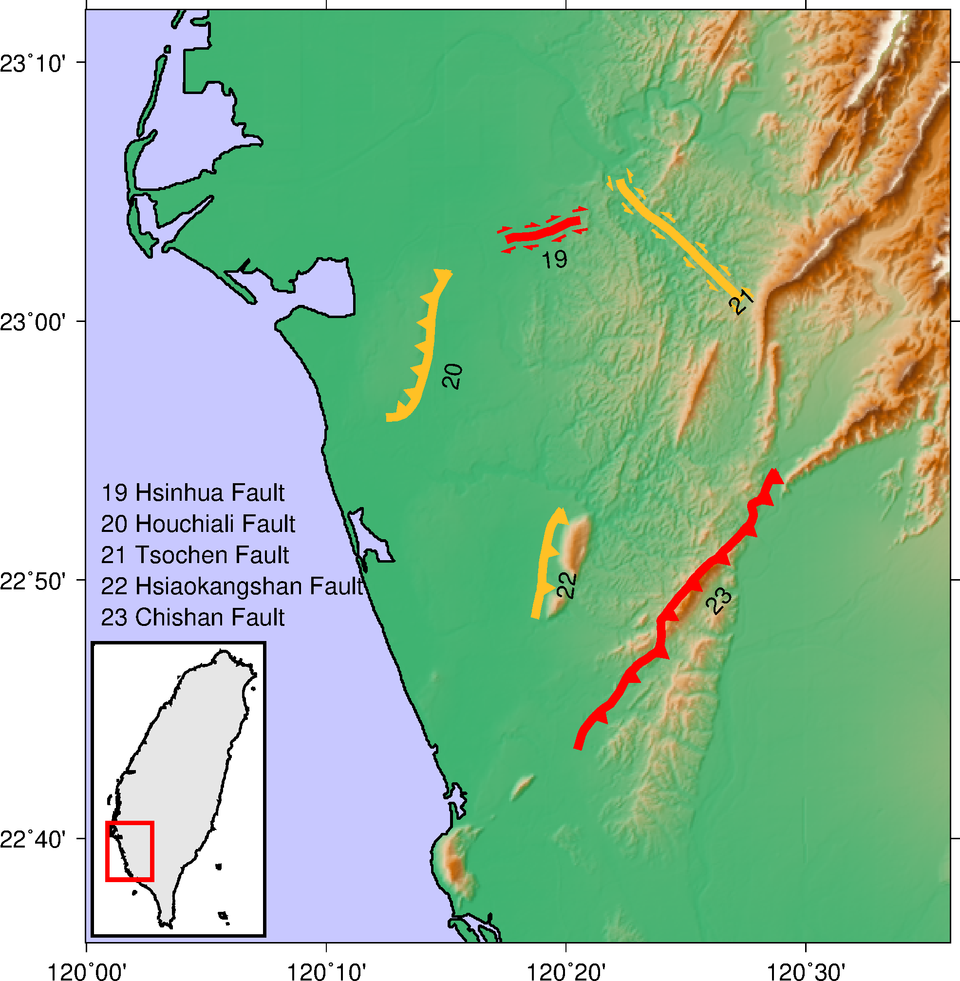
接下來是示範如何繪製不同的斷層型態。

完成圖如下:

批次檔

set ps=11_6_fault_type.ps
set data=D:\GMT_data\
set cpt=dem3.cpt

gmt psbasemap -R120.0/120.6/22.6/23.2 -JM15 -BWeSn -Ba -P -K --MAP_FRAME_TYPE=plain > %ps%
gmt grdimage %data%tw_40.grd -R -JM -C%cpt% -I%data%tw_40shad.grd -K -O >> %ps%
gmt pscoast -R -JM -Df -W1 -S200/200/255 -K -O >> %ps%

# 新化 右移斷
gmt gmtconvert %data%CGS_fault.gmt -S"Hsinhua Fault" > tmp
gmt psxy tmp -R -JM -W4,red -Sf.5/.2+r+s+p1,red -K -O >> %ps%
# 後甲里 逆移斷 西傾
gmt gmtconvert %data%CGS_fault.gmt -S"Houchiali Fault" > tmp
gmt psxy tmp -R -JM -W4,255/193/37 -Sf.4/.25+r+t+o.12+p1,255/193/37 -G255/193/37 -K -O >> %ps%
# 左鎮 左移斷
gmt gmtconvert %data%CGS_fault.gmt -S"Tsochen Fault" > tmp
gmt psxy tmp -R -JM -Sf.7/.2+l+s+p1,255/193/37 -K -O >> %ps%
gmt gmtconvert %data%CGS_fault.gmt -S"Tsochen Fault" > tmp
gmt psxy tmp -R -JM -W4,255/193/37 -K -O >> %ps%
# 小崗山 逆移斷 東傾
gmt gmtconvert %data%CGS_fault.gmt -S"Hsiaokangshan Fault" > tmp
gmt psxy tmp -R -JM -W4,255/193/37 -Sf.7/.25+l+t+o.12+p1,255/193/37 -G255/193/37 -K -O >> %ps%
# 旗山斷層 逆移兼 東傾
gmt gmtconvert %data%CGS_fault.gmt -S"Chishan Fault" > tmp
gmt psxy tmp -R -JM -Sf.7/.25+l+t+o.12+p1,red -Gred -K -O >> %ps%
gmt gmtconvert %data%CGS_fault.gmt -S"Chishan Fault" > tmp
gmt psxy tmp -R -JM -W4,red -K -O >> %ps%

awk "$4<=25 {print $0}" fault_label_fix.dat | ^
gmt pstext -R -JM -F+f12+a -D.4/-.4 -K -O >> %ps%

gmt gmtconvert -L %data%CGS_fault.gmt > tmp
sed -i 's\\"\\\\g' tmp
awk "{print $7, $8, $2}" tmp > tmp2
awk "NR !=1 {print 120.01, 23.25, $4}" fault_label_fix.dat > tmp1
awk "NR==FNR{tmp1[$3]=$0; next} {$3=tmp1[$3]; print}" tmp2 tmp1 > tmp3
awk "NR>=19 && NR <=23 {print $1, $2-($5-1)*.02, $5, $3, $4}" tmp3 | ^
gmt pstext -R -JM -F+f12p+jML -K -O >> %ps%

gmt pscoast -R119.8/122.1/21.8/25.4 -JM3 -Df -W1 -B0 -S255 -G230 ^
-X.1 -Y.1 -K -O --MAP_FRAME_TYPE=plain >> %ps%
gmt psbasemap -R -JM -D120.0/120.6/22.5/23.2 -F+p2,red -K -O >> %ps%

gmt psxy -R -J -T -O >> %ps%
gmt psconvert %ps% -Tg -A -P
del tmp*

學習到的指令:

• psxy -Sf.7/.25+l+t+o.12+p1,red在線段中側邊繪製一個圖案， 用法是-Sfgap[/size][+l|+r][+b+c+f+s+t][+ooffset][+p[pen]]
  • +l圖案繪製在線段左側；+r圖案繪製在線段右側。
  • +t圖案是三角形、+b矩形、+c圓形、+f斷層、+s滑移箭頭。
  • +o圖案起始的偏移量。
  • +p圖案的邊框筆觸。

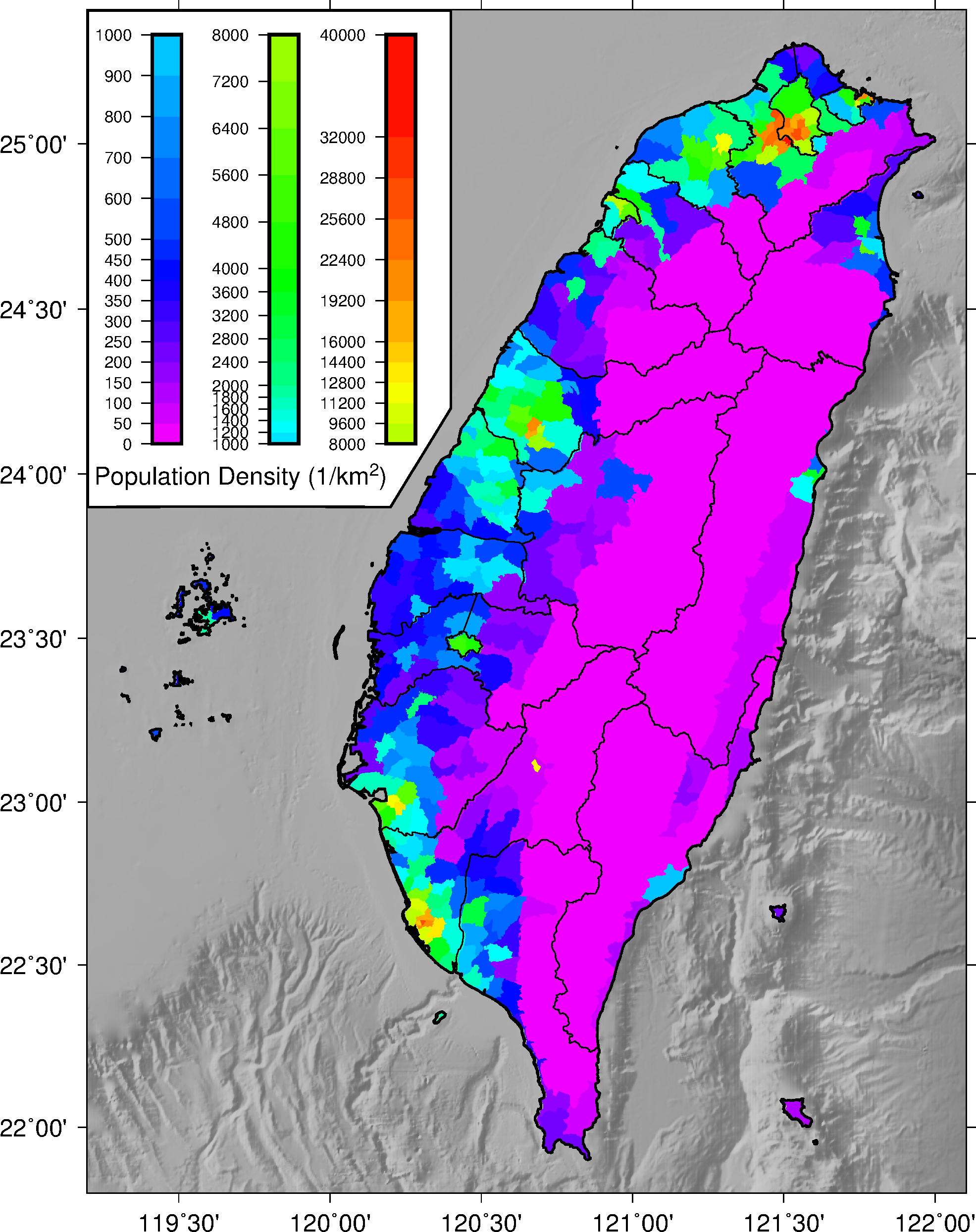
11.7 人口密度

本章最後一小節，將利用人口密度資料，來示範區塊文件如何配合psxy -C指令，來完成人口密度分佈圖。

使用的資料檔:

• 鄉鎮人口密度
• 色階檔分隔條件
• 人口密度色階檔

完成圖如下:

批次檔

set ps=11_7_population_density.ps
set data=D:\GMT_data\
set cpt=rainbow.cpt

# population density map
gmt psbasemap -R119.2/122.1/21.8/25.4 -JM15 -BWeSn -Ba -P -K --MAP_FRAME_TYPE=plain > %ps%
gmt grdimage %data%tw_500_119.grd -R -JM -C%cpt% -I%data%tw_500shad_119.grd -M -K -O >> %ps%
gmt pscoast -R -JM -Df -Gc -K -O >> %ps%
# gmt makecpt -C%cpt% -Trange.txt -D -Fr > tmp.cpt
# awk "{print $0}" range.txt | gmt makecpt -C%cpt% -E42 -D -Fr > tmp.cpt2
gmt psxy %data%country_popuDen_2016f.gmt -R -JM ^
-Cpopulation_density.cpt -L -K -O >> %ps%
gmt psxy %data%city_2016.gmt -R -JM -W.5 -K -O >> %ps%
gmt pscoast -R -JM -Df -Q -K -O >> %ps%
gmt pscoast -R -JM -Df -W1 -K -O >> %ps%

# legend set
echo 119.2 25.4 > tmp
echo 119.2 23.9 >> tmp
echo 120.2 23.9 >> tmp
echo 120.4 24.2 >> tmp
echo 120.4 25.4 >> tmp
gmt psxy tmp -R -JM -G255 -W1 -L -K -O >> %ps%
awk "$1>=0 && $1< 1000 {print $0}" population_density.cpt > tmp.cpt
gmt psscale -Ctmp.cpt -R -JM -Dx1.1/12.8+w7/.5 -A -S ^
-K -O --FONT_ANNOT_PRIMARY=8p >> %ps%
awk "$1>=1000 && $1< 8000 {print $0}" population_density.cpt > tmp.cpt
gmt psscale -Ctmp.cpt -R -JM -Dx3.1/12.8+w7/.5 -A -S ^
-K -O --FONT_ANNOT_PRIMARY=8p >> %ps%
awk "$1>=8000 && $1< 40000 {print $0}" population_density.cpt > tmp.cpt
gmt psscale -Ctmp.cpt -R -JM -Dx5.1/12.8+w7/.5 -A -S ^
-K -O --FONT_ANNOT_PRIMARY=8p >> %ps%
echo 119.22 24.00 Population Density (1\057km@+2@+) | ^
gmt pstext -R -JM -F+f12,0+jML -K -O >> %ps%

gmt psxy -R -J -T -O >> %ps%
gmt psconvert %ps% -Tg -A -P
del tmp*

學習到的指令:

• #符號開頭的兩行makecpt ... -Trange.txt -Fr+c ...及... -E42 ...。
  • -Trange.txt用range.txt來指定色階檔分隔的依據。
  • -Fr指定輸出為RGB格式。
  • -E42讀取資料最後一欄，找出最大最小值，42表示色階分隔數量。
• 會分兩次製作色階檔是因為，想製作非線性的間隔，先製作非線性排序的色階檔(tmp.cpt)， 接著製作同範圍的線性色階檔(tmp.cpt2)，再手動將非線性排序的間隔取代線性色階檔的間隔， 用此方式來達到非線性的色階檔。
• 打開country_popuDen_2016f.gmt會發現，在區塊檔頭的地方，出現-Z100之類的訊息， 原來GMT在讀取區塊檔頭資訊時，透過-Z會自動將這區塊內的資料賦予Z軸值為100， 借此-C就會依照Z軸的值來填色，-L是確保區塊中資料是封閉多邊形。
• psscale ... -A -S ...。
  • -A讀取色階檔裡面的間隔當作刻度。
  • -S不繪製色階中黑色的區隔線。
• echo 119.22 24.00 Population Density (1\057km@+2@+)， \057對應特殊字元\，@+2@+則是寫出上標數字2。

11.8 參考批次檔

列出本章節使用的批次檔，供讀者參考使用，檔案路經可能會有些許不同，再自行修改。

• 11_3_taiwan_road
• 11_4_region_border
• 11_5_drainage_area
• 11_6_cgs_fault
• 11_6_fault_type
• 11_7_population_density

---

上一章 – 下一章